MFP is an approach to multivariable model-building which retains continuous predictors as continuous, finds non-linear functions if sufficiently supported by the data, and removes weakly influential predictors by backward elimination (BE).

The main issues of the approach arise from the two key components:

• variable selection with backward elimination and

• selection of an FP function to model non-linearity

1. Motivating example

Multivariable model–building with continuous predictors

Should we assume linear functional relationships or check whether a non-linear function fits substantially better?

Influence of 7 potential predictors of log prostate-specific antigen (log PSA) in 97 patients with prostate cancer. A linear regression model (normal-errors regression) seems sensible as the outcome, log PSA, is continuous. For more details see Appendix A.2.5 in our book.

The two main questions are:

• include all variables and estimate corresponding parameters, or eliminate variables with at most weak effects?
• assume linear relationships or allow non-linear functions?

Decisions depend on the aim of the model: prediction or explanation? Prediction aims to predict the outcome as accurately as possible, with little regard for the detailed components of the model; explanation seeks a good fit to the data, but further demands interpretable functions, and a model that as far as possible is consistent with subject-matter knowledge. Generally, our stance is that explanation is the more informative approach.

In what follows, the term ‘full model’ means the model that includes all candidate predictors, whether statistically significant or not, and retains all continuous predictors as linear functions. BE(0.05) means the linear model selected by backward elimination at the 0.05 significance level. MFP(0.05) means the MFP model with functions and variables selected at the 0.05 significance level. It is also possible using different significance level for the two components. MFP(0.05, 0.01)  means that variables are selected at 0.05 and functions at 0.01 level. Furthermore, it is possible choosing specific significance levels for each variable.

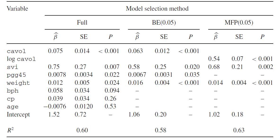
The table below shows the results for the full, BE(0.05) and MFP(0.05) models.

Reproduced from R&S (2008) with permission from John Wiley & Sons Ltd.

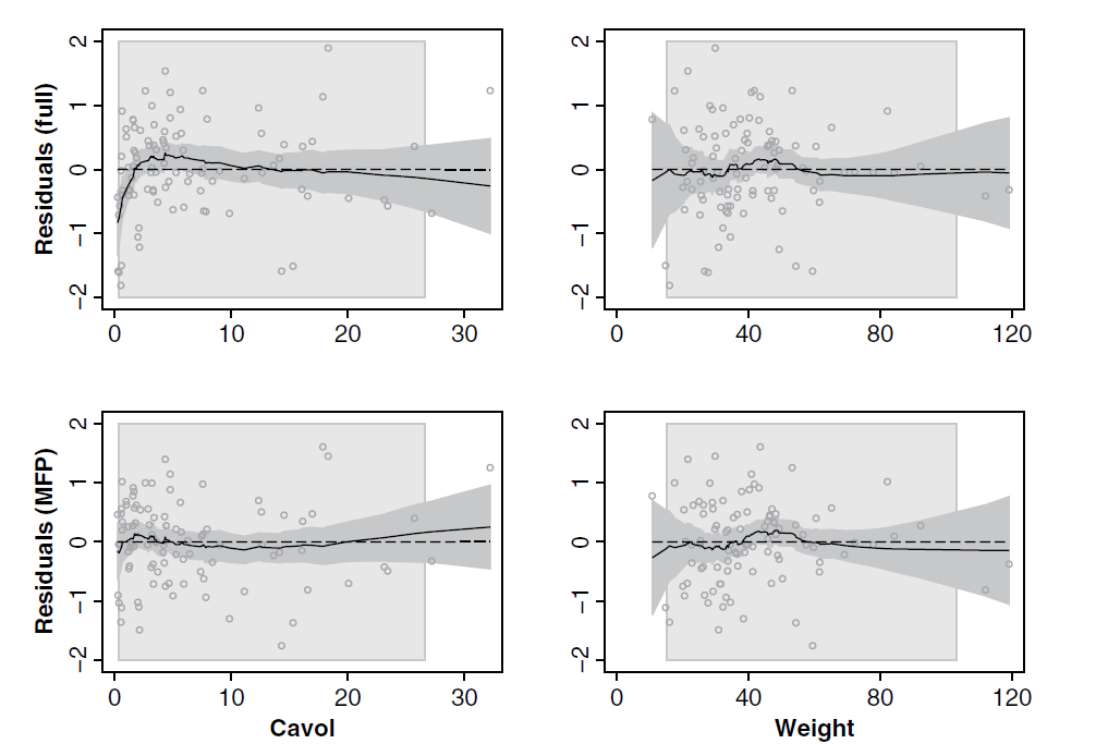
The full model is the starting point for both BE and MFP. BE(0.05) eliminates 3 of the 7 variables. R² as a measure of explained variation is only slightly reduced by removing 3 variables. MFP selects a non-linear (log) function for the variable cavol (cancer volume) and eliminates four variables. For details see below. Although the MFP model includes only 3 variables, its R² is slightly larger than that from the full model. Residual plots indicate that the full model does not fit small cavol values well:

The figure shows plots of residuals comparing the fit of the full and MFP models to log PSA. The upper panels show the full model and the lower panels the MFP model. Residuals and smoothed residuals with 95 percent pointwise confidence intervals are plotted against cavol on the left and weight on the right.

Reproduced from R&S (2008) with permission from John Wiley & Sons Ltd.

 

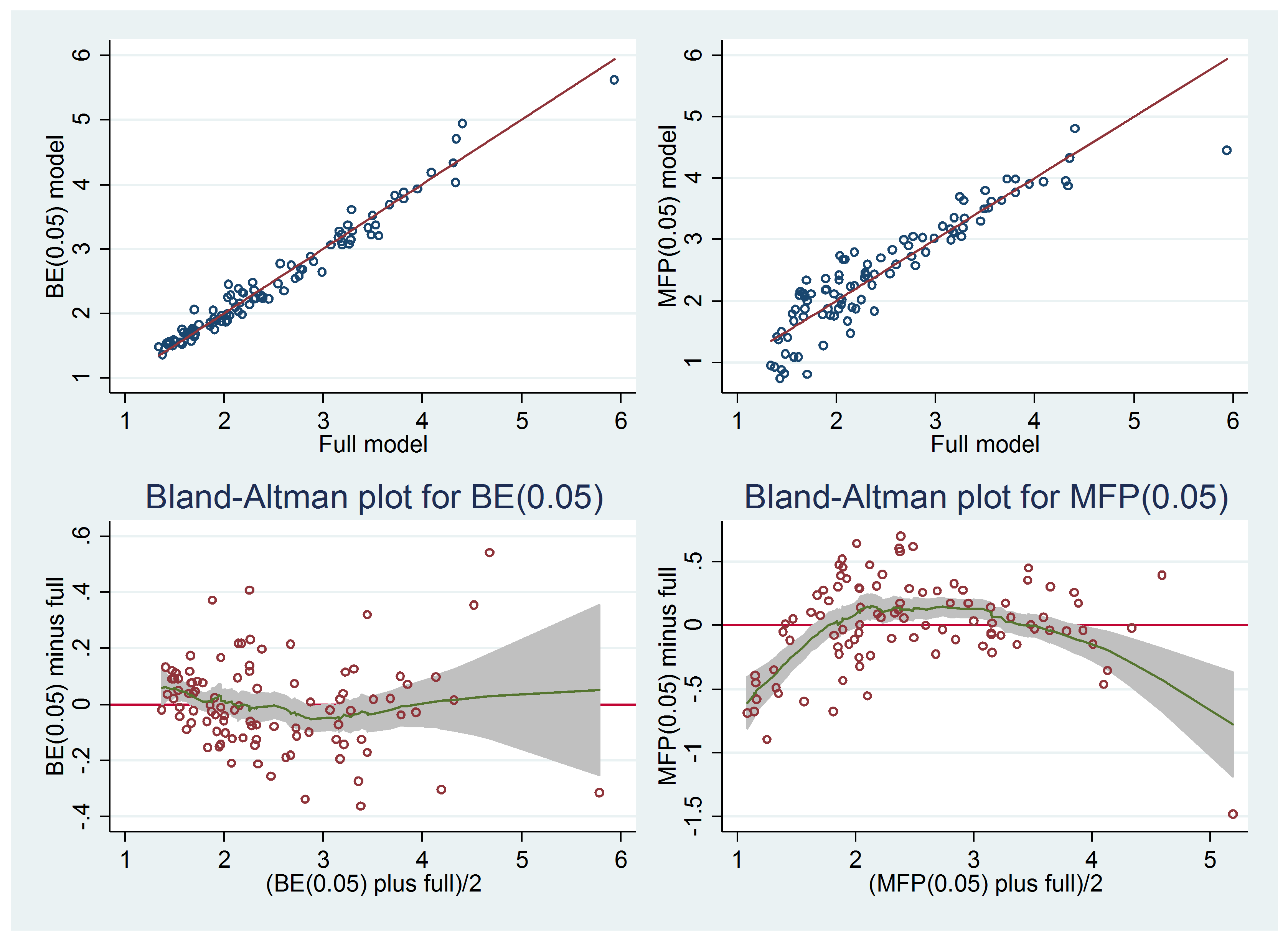
In the following plots we compare predictors from the full, the BE(0.05)  and the MFP(0.05) model. As indicated by the R² values and shown below, predictors from all three models are similar. However, for explanatory purposes the MFP model seems to be most appropriate. Its fit for very low cavol values is much better (see figure above) and it includes only 3 variables in contrast to the full model with 7 variables, some of them with  hardly any effect on the outcome. This becomes obvious by the comparison of the full model with the BE(0.05) model in which 3 of the 7 variables are eliminated without substantial loss in R². However, using this full model to predict the outcome for a new patient all 7 variables are required.

We show scatterplots and plots with raw and smoothed residuals. The plots on the left side compare predictors from the full model with the BE(0.05) model. The scatterplot and the Bland-Altman plot show that they are very similar. Using BE to eliminate variables with weak effects hardly affects the predictor. In contrast, predictors from the full model and the MFP model differ more, as well illustrated by the two plots on the right side. The smoothed residuals in the Bland-Altman plot clearly exhibit that the difference between the two predictions depend on the value of the predictor. Such a large difference is not obvious by simply comparing R² values of these two models. 

2. The MFP algorithm - basic concept

Using the prostate example we briefly explain, how the algorithm works. Like backward elimination it starts with the full model and investigates whether variables can be eliminated. However, for each of the continuous variables the function selection procedure (FSP) is used to check whether a non-linear function fits the data significantly better than a linear function. After a first cycle some variables will be eliminated and for some continuous variables a better fitting non-linear function may have been determined. The algorithm starts a second cycle, but the new starting model now has less variables (as some were eliminated) and perhaps non-linear functions for some of the continuous variables. In the second cycle all variables will be reconsidered (even if they were not significant at the end of the first cycle) and FSP is used again to determine the ‘best’ fitting FP function (it may be different because other ‘adjustment’ variables are in the model). This yields the result of cycle 2 which is the starting model for cycle 3. In most cases the model does not change anymore in cycle 3 or 4 and the algorithm stops with the final MFP model.   

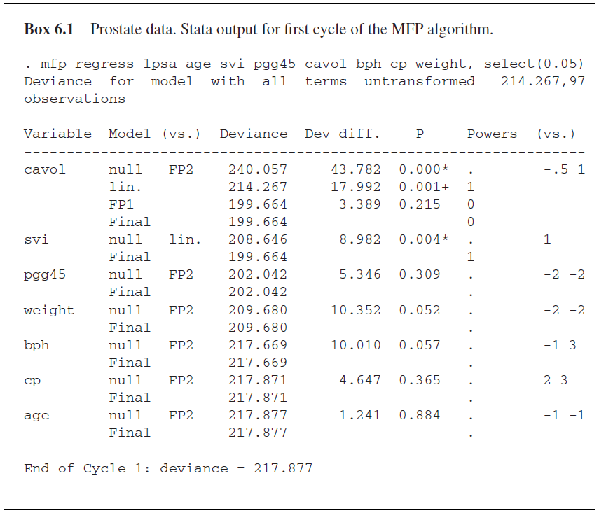
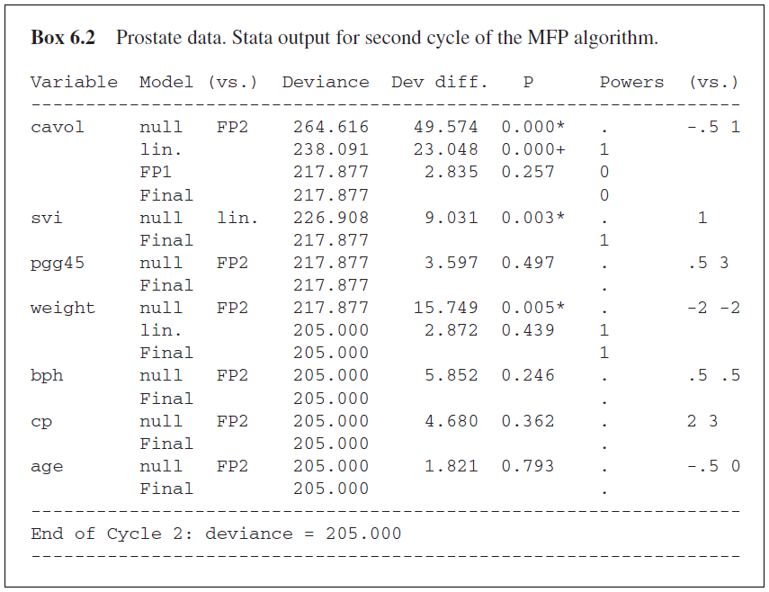
Important is the order of ‘searching’ for model improvement by better fitting non-linear functions. Obviously, mismodelling the functional form of a variable with a strong effect is more critical than mismodelling the functional form of a variable with a weak effect. Therefore the order is determined by p-values in the full model. Variables with a small p-value are considered first. Boxes 6.1 and 6.2 from our book illustrate the algorithm for the prostate data. We use 5% for both variable elimination and function selection.

Reproduced from R&S (2008) with permission from John Wiley & Sons Ltd.

The order is given by p-values in the full model (<0.001 for cavol,…, 0.53 for age.) Adjusting for other variables and functions currently in the model (all six variables svi – age, functions all linear) a suitable function for cavol is selected by the FSP. The best FP2 function fits significantly better than null (elimination of the variable) and also than linearity. The comparison of the best FP2 with the best FP1 function is no longer significant (p=0.215) and FP1 is selected. The power is ‘0’ which means log(cavol). Next svi is checked in a model including log(cavol) (log function just selected) and the other five variables pgg45, …,age still in the model. Svi is binary and there is only one test which is significant (p=0.004). Svi remains in the model. In the next step the continuous variable pgg45 is assessed in the same model as for svi. The p-value in the first step (FP2 versus null) is non-significant (p=0.309) and the variable is eliminated for the following steps of the cycle. Therefore the effect of weight is investigated in a model adjusting for log(cavol), svi and the three variables bph, cp, age which come below weight. For weight the first test is non-significant (p = 0.052) and the variable is eliminated for the rest of the cycle. In the following steps bph, cp and age are also eliminated and in the first cycle a simple model including log(cavol) and svi is selected.
This is the new starting model for the second cycle. The effect of cavol is investigated again, but now in a simple model adjusting for svi only. Deviances are larger than in cycle 1 (because the five variables pgg45 – age do no longer belong to the ‘adjustment’ model) but FSP, which uses p-values based on deviance differences, selects log(cavol) again. Investigations for svi and pgg45 confirm that svi should be in and pgg45 should be out of the model. Weight is the variable considered next. In contrast to the first cycle the test for inclusion (FP2 vs null) is significant (p=0.005) and weight needs to be re-included in the model. The second test of the FSP (FP2 vs linearity) is non-significant and a linear function is chosen for weight. In following steps bph, cp and age are investigated in models adjusting for log(cavol), svi (binary) and weight (linear). Compared to the first cycle p-values change but all are much larger than 0.05. None of these variables are included and cycle 2 ends with the model log(cavol), svi (binary) and weight (linear).
This model is the new starting model for cycle 3 where all seven variables are investigated again. There are no further changes and cycle 3 ends with the same model as cycle 2. The algorithm stops. Parameter estimates and residual plots of the selected MFP(0.05,0.05) model with cavol(0), svi and weight(1) are given above.

3. MFP modelling - philosophy and related matters

For a detailed description of the algorithm and some relevant issues see Section 6 MFP: Multivariable Model-Building with Fractional Polynomials. There are 4 headings in the discussion (Philosophy of MFP; Function Complexity, Sample Size and Subject-Matter Knowledge; Improving Robustness by Preliminary Covariate Transformation; Conclusion and Future).

For readers with different levels of methodological knowledge we have published three papers about MFP modelling:

• S&R (1999): Building multivariable prognostic and diagnostic models: Transformation of the predictors by using fractional polynomials

• Royston et al (1999): The use of fractional polynomials to model continuous risk variables in epidemiology

• Sauerbrei et al (1999): Modelling the effects of standard prognostic factors in node positive breast cancer

The first article is methodological in character whereas the other two have more of an applied flavour. There are some philosophical thoughts on our way of thinking about variable and function selection and the role of MFP in Sauerbrei et al (2007): Selection of important variables and determination of functional form for continuous predictors in multivariable model building. Based on these thoughts and our extensive experience we have created a table giving some guidance for model building by selection of variables and functional forms for continuous predictors under some assumptions.
The table has been adapted in section 12.2 Towards Recommendations for Practice of our book.

Guidance documents are currently discussed in topic group 2 Selection of variables and functional forms in multivariable analysis of the STRATOS (STRengthening Analytical Thinking for Observational Studies) initiative. For a summary of the motivation, mission, structure and main aims see Sauerbrei et al (2014).

More mathematical descriptions of MFP are published in the International Encyclopedia of Statistical Science (S&R (2011): Multivariable Fractional Polynomial Models) and in Wiley StatsRef (S&R (2016): Multivariable Fractional Polynomial Models).
Issues of MFP modelling are also described in R&S (2005): Building multivariable regression models with continuous covariates in clinical epidemiology, with an emphasis on fractional polynomials.
For a less technical description see S&R (2010): Continuous Variables: To Categorize or to Model?. Based on the structure of the German Breast Cancer Study Group (GBSG) data, used in several papers, we have created ART (an artificial dataset) and discuss issues of MFP modelling in detail (Chapter 10 How To Work with MFP).
This simulated dataset has the major advantage that the ‘truth’ is known.

4. Effects of influential points and sample size on the selection and replicability of MFP models

Influential points (IPs) and small sample sizes can both have a strong impact on a selected function and MFP model.

• Using the simulated data from the ART study (six continuous and four categorical predictors; normal-errors regression; see Chapter 10), Sauerbrei et al (2023) illustrate approaches which  can help to identify IPs with an influence on function selection and the MFP model. The results showed that one or more IPs can drive the functions and models selected,specifically for smaller sample size. However, when the sample size was relatively large and regression diagnostics were carefully conducted, MFP selected functions or models that were similar to the underlying true model (see also FP - 4.2).

 

True function and functional form selected in datasets with sample sizes 125, 250 and 500 (minus some identified influential points). The continuous variable x7 has no effect and was never selected.

True function and functional form selected in three independent datasets with sample size 500 (minus some identified influential points). The continuous variable x7 has no effect and was never selected.

 

5. Comparison with splines

To select a suitable function for a continuous variable, spline-based functions are the most important competitors. By replacing the FP component of MFP with splines, we have developed the procedures MVRS (9.3 MVRS: A Procedure for Model Building with Regression Splines) and MVSS (9.4 MVSS: A Procedure for Model Building with Cubic Smoothing). Software in Stata has been made available (R&S (2007): Multivariable modelling with cubic regression splines: A principled approach.

MFP and model-building using multivariable splines are compared in examples (Sauerbrei et al (2007): Selection of important variables and determination of functional form for continuous predictors in multivariable model building; chapter 9 Some Comparisons of MFP with Splines) and in a large simulation study (Binder et al (2013): Comparison between splines and fractional polynomials for multivariable model building with continuous covariates: a simulation study with continuous response).

Conclusions from the simulation study are:

5.4 Final conclusions The  main  conclusions  about  the  different  types  of  modelling  procedures  we  have  studied  in  a multivariable framework are as follows: With a relatively small amount of information, a suitable explanatory model cannot be obtained. Prediction performance from all types of models derived, with or without selection, linear or nonlinear, is similar. With a medium amount of information, MFP performs better than splines in several criteria. However, we recognize that splines can model some functions that cannot be reasonably approximated by members of the FP2 class. For a large amount of information and no function with local structure, MFP and our versions of restricted cubic and penalized splines often select similar models. In addition to the aforementioned conclusions that are directly derived from the results of our simulations, it should be noted that MFP models are easier to implement than splines. Specifically, the absence of clear guidelines regarding the criteria for selecting a multivariable spline model appropriate for a given application is an important barrier against their more widespread use in real-life analyses. Reproduced from Binder et al. (2013), with permission from John Wiley & Sons Ltd.

Naturally, a full understanding requires reading the paper in detail.

 

6. Stability of models derived with MFP

In one example dataset, we have investigated the stability of variables and functions selected with the MFP approach. (8.7 Model Stability for Functions; 8.8 Example 4: GBSG Breast Cancer Data; 8.9 Discussion)
See also R&S (2003): Stability of multivariable fractional polynomial models with selection of variables and transformations: a bootstrap investigation
Similar investigations can also be found for a model derived with splines (Binder & Sauerbrei (2009): Stability analysis of an additive spline model for respiratory health data by using knot removal).